


単回帰分析とは
回帰係数が1つで独立変数が1つ
下の式で表せる回帰を単回帰という。
$$ y = \beta_0 + \beta_1 x$$
中学校でやった1次関数の形です。
Pythonで単回帰分析
stats.linregress(x, y)で単回帰
線形単回帰は、stats.linregress(x, y)を使います。
scipyから、statsをインポートします。
このメソッドを通すと、
- 傾き
- 切片
- 相関係数
- P値(t検定で使う)
- 推定勾配の標準誤差
の順で値が返ってきます。
Standard error of the estimated gradient.を直訳しただけなので、この推定勾配の標準誤差はなんのことかわかりません。飛ばします。
ソースコード
import numpy as np
from pylab import *
from scipy import stats
#ランダムな数を固定
np.random.seed(0)
x = np.random.normal(3.0, 1.0, 100)
y = 10 + x * np.random.rand(100)
#散布図
sc = scatter(x, y)
plt.show(sc)
'''
単回帰
'''
slope, intercept, r_value, p_value, std_err = \
stats.linregress(x, y)
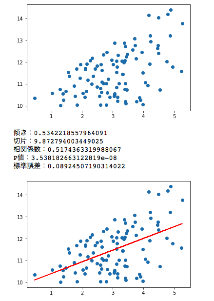
print("傾き:{0}\n切片:{1}\n相関係数:{2}\nP値:{3}\n\
標準誤差:{4}".format(slope,intercept, r_value, p_value,std_err))
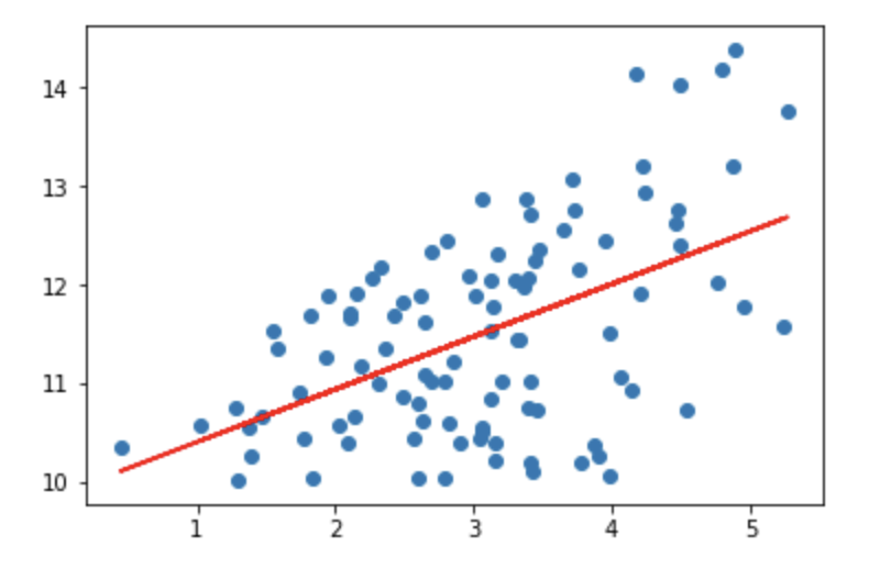
#直線を描く
fitline = slope * x + intercept
plt.scatter(x, y)
plt.plot(x, fitline, c='r')
plt.show()
出力結果
sklearnのLinearRegressionで単回帰
sklearnのLinearRegressionで単回帰を実行します。
LinearRegressionの場合は、P値は算出されません。
ソースコード
import numpy as np
import matplotlib.pyplot as plt

#ランダムな数を固定
np.random.seed(0)
x = np.random.normal(3.0, 1.0, 100)
y = 10 + x * np.random.rand(100)

x = x.reshape(-1, 1)
y = y.reshape(-1, 1)


#回帰係数を計算
from sklearn.linear_model import LinearRegression

lr = LinearRegression().fit(x, y)

slope = lr.coef_
intercept = lr.intercept_

#直線を描く
fitline  = slope * x + intercept
plt.scatter(x, y)
plt.plot(x, fitline, c='r')
plt.show()
出力