


elastic net
Pythonでelastic netを実行していきます。
elastic netは、sklearnのlinear_modelを利用します。
インポートするのは、以下のモジュールです。
from sklearn.linear_model import ElasticNet
elastic net回帰
説明変数の中に非常に相関の高いものがるときにはそれらの間で推定が不安定になることが知られている。
これは、多重共線性として知られている。
この多重共線性が生じる場合、正則化項として、ridge回帰とlasso回帰で用いる正則化項の両方を使う方法をelastic netという。
sklearnのelastic net回帰
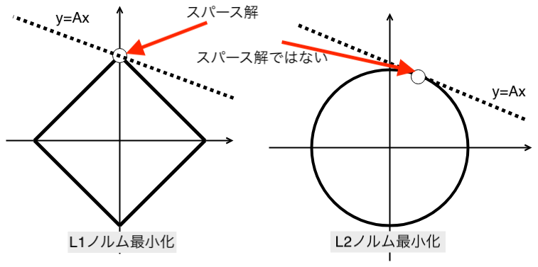
L1ノルムの割合をαとし、L2ノルムの割合を(1-α)と設定する。
$$min \left[ \Vert y – \displaystyle \sum_{ j }^{ } \beta_jx_i^{j} \Vert_2^2 + \lambda( \alpha \Vert \beta \Vert_1 + (1-\alpha) \Vert \beta \Vert_2^2 ) \right]$$
sklearnでは、引数alphaは上の式のλ、l1_ratioはαとなっていることに注意が必要である。
最適化は、
1 / (2 * n_samples) * ||y - Xw||^2_2

+ alpha * l1_ratio * ||w||_1

+ 0.5 * alpha * (1 - l1_ratio) * ||w||^2_2
公式サイト

Pythonプログラム
係数を表示するプログラムです。
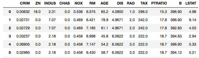
データには、ボストンデータを使います。
Xの変数は、13個の重回帰式になります。
elastic-netを実行していきましょう。
ソースコード
import pandas as pd
import matplotlib.pyplot as plt
import numpy as np
from sklearn.linear_model import ElasticNet
from sklearn.datasets import load_boston

# サンプルデータを用意
dataset = load_boston()

# 説明変数データを取得
data_x = pd.DataFrame(dataset.data, columns=dataset.feature_names)

#被説明変数データを取得
data_y = pd.DataFrame(dataset.target, columns=['target'])


#データの
print("説明変数行列のサイズ:{}".format(data_x.shape[1]))
print("被説明変数のサイズ:{}".format(data_y.shape))
print("説明変数の変数の個数:{}".format(data_x.shape[1]))
coef_n = data_x.shape[1]

decimal_p = 3

#ElasticNet
elastic_net = ElasticNet(alpha = 0.5).fit(data_x, data_y)
print(elastic_net.coef_.round(decimal_p))
結果
[-0.092 0.054 -0.032 0. -0. 1.722 0.009 -0.99 0.311 -0.016
-0.804 0.009 -0.707]
参考