


RNNとは
リカレントニューラルネットワーク
時系列データを扱う「時間」という概念を取り入れたニューラルネットワーク
LSTMやGRUという手法がある。
降水量、株価、為替などが時系列データにあたる。
LSTM
Long-Short-Term-Memoryの略
長期・短期の時間依存性を保つ。
RNNの実践
Udemyの講座のDeep Learning A-Z™: Hands-On Artificial Neural Networksを参考にしています。
プログラム
上で紹介されているプログラムを少し書き換えて、処理を軽くしています。
具体的には、
- LSTMの層を減らしました
- エポック数を偉しました
- 全結合層を1層足しました
この3点を変更しました。
ソースコード
import numpy as np
import matplotlib.pyplot as plt
import pandas as pd
# 訓練データ
dataset_train = pd.read_csv('Google_Stock_Price_Train.csv')
training_set = dataset_train.iloc[:, 1:2].values
# Feature Scaling
from sklearn.preprocessing import MinMaxScaler
sc = MinMaxScaler(feature_range = (0, 1))
training_set_scaled = sc.fit_transform(training_set)
# Creating a data structure with 60 timesteps and 1 output
X_train = []
y_train = []
for i in range(60, 1258):
X_train.append(training_set_scaled[i-60:i, 0])
y_train.append(training_set_scaled[i, 0])
X_train, y_train = np.array(X_train), np.array(y_train)
# Reshaping
X_train = np.reshape(X_train, (X_train.shape[0], X_train.shape[1], 1))
#RNNの構築
# Keras
from keras.models import Sequential
from keras.layers import Dense
from keras.layers import LSTM
from keras.layers import Dropout
# Initialising the RNN
regressor = Sequential()
# Adding the first LSTM layer and some Dropout regularisation
regressor.add(LSTM(units = 50, return_sequences = True, input_shape = (X_train.shape[1], 1)))
regressor.add(Dropout(0.2))
regressor.add(LSTM(units = 50))
regressor.add(Dropout(0.2))
# Adding the output layer
regressor.add(Dense(units = 20))
regressor.add(Dense(units=1))
# Compiling the RNN
regressor.compile(optimizer = 'adam', loss = 'mean_squared_error')
# Fitting the RNN to the Training set
regressor.fit(X_train, y_train, epochs = 20, batch_size = 32)
# Part 3 - Making the predictions and visualising the results
# Getting the real stock price of 2017
dataset_test = pd.read_csv('Google_Stock_Price_Test.csv')
real_stock_price = dataset_test.iloc[:, 1:2].values
# Getting the predicted stock price of 2017
dataset_total = pd.concat((dataset_train['Open'], dataset_test['Open']), axis = 0)
inputs = dataset_total[len(dataset_total) - len(dataset_test) - 60:].values
inputs = inputs.reshape(-1,1)
inputs = sc.transform(inputs)
X_test = []
for i in range(60, 80):
X_test.append(inputs[i-60:i, 0])
X_test = np.array(X_test)
X_test = np.reshape(X_test, (X_test.shape[0], X_test.shape[1], 1))
predicted_stock_price = regressor.predict(X_test)
predicted_stock_price = sc.inverse_transform(predicted_stock_price)
# Visualising the results
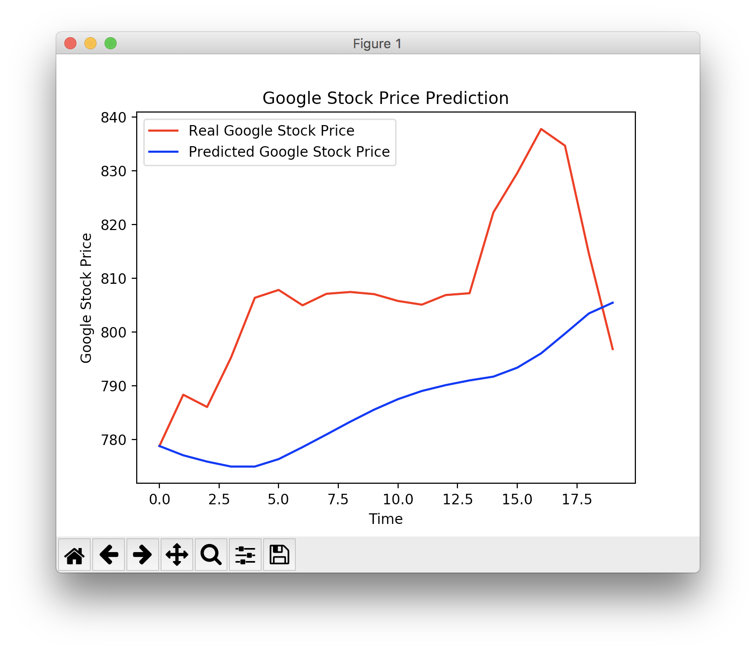
plt.plot(real_stock_price, color = 'red', label = 'Real Google Stock Price')
plt.plot(predicted_stock_price, color = 'blue', label = 'Predicted Google Stock Price')
plt.title('Google Stock Price Prediction')
plt.xlabel('Time')
plt.ylabel('Google Stock Price')
plt.legend()
plt.show()
結果